Method behind AnimalGAN

A generative adversarial network model alternative to animal studies for clinical pathology assessment | Nature Communications – Xi Chen, Ruth Roberts, Zhichao Liu & Weida Tong , 2023 

The source of the data:

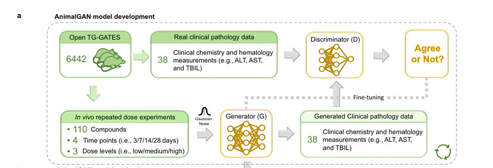
• AnimalGAN was trained using Open TG-GATEs, a large, publicly available toxicology database that stores both: Traditional toxicology data and Toxicogenomic profiles.
• The data comes from experiments where animals (and cells) were exposed to ~170 different compounds at different doses and time points. From this they narrowed findings to clinical pathology, specifically looking at 38 biological measurements across 4 time points of 3, 7, 14 and 28 days.
• AnimalGAN can be used widely but the paper specifically focuses on its usage for liver abnormalities. The model learned from over 8,000 rats across 1600+ treatment conditions. Essentially this becomes the biological blueprint in which the AI tries replicates.
  

From chemicals to numbers:

• Each chemical compound was translated into a numerical format using:
  • PubChem CID, Structure Data Files (SDF) and SMILES strings (a text-based way to represent molecules)
• these were then processed using a Python tool called Mordred, which generated:
  • 1,826 molecular descriptors per compound, which captures both 2D and 3D structural features. This step is critical since it links what a chemical looks like to what it does biologically.

Generator vs. Discriminator – competing AIs

• AnimalGAN has two neural networks: A generator (G) → creates synthetic biological data, and A discriminator (D) → tries to distinguish real data from fake
  • The generator takes a condition (C) (compound + dose + time) + random noise (Z) and produces simulated clinical pathology data (X).
  • The discriminator then compares real experimental data vs generated (fake) data, and essentially tries to tell them apart.
  • As the system trains the generator gets better at fooling the discriminator and the discriminator gets better at detecting fakes
  • Once the models converge and the discriminator can’t tell the difference anymore, the model is trained.

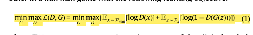
• The formula below is for VanillaGAN, G and D iteratively being trained against one another.
  • E[.] represents expectation
  • x is a vector of the clin path measurements sampled from the distribution of the real data which is Preal . Z is a vector with random noise sampled from a Gaussian distribution Pz.

• The formula below is for ConditionalGAN (cGAN) and its meant to develop data within a specific condition. The main difference is that both the generator and discriminator have condition as one of the inputs. The problem was that cGAN would be unstable as it played the discriminator min/max game given the small training sample size.

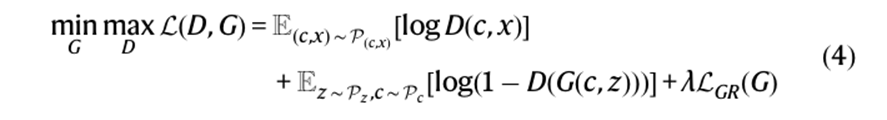
• WassersteinGAN (WGAN) uses the Wasserstein distance also called the Earth Mover (EM) as an explicit way to measure the distribution divergence in the loss function to overcome gradient disappearance to partially alleviate the mode collapse. It basically was a more stable way of mreasuring differences between real and fake data. AnimalGAN uses both cGAN and WGAN, cGAN allows for generation of clin path measures at a given condition while WGAN improves the convergence of the model.
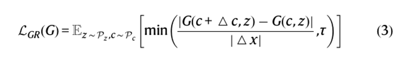
• A regularization term was used called Lipschitz regularization (formula below) which was implanted onto generator loss to improve the generalizability of the generator. This allowed the generator to balance neighboring conditions in continuous space without losing the importance of the input conditions through Lipschitz regularization along with interpolations of conditions pairs. This way when the system was given new conditions, the regularization term allows for data to be generated based on similar conditions and structures.

The final formula for AnimalGAN became

Generator architecture, the components

• It receives 4 inputs, with the first 3 as conditions c= concat(s,d,t)
  • s → chemical structure (1826 dimensional vector of molecular representation by using Mordred),
  • d → dose level (low, medium, high; ratio 1:3:10), with the high dose equal to MTD determined in a 7 day dose study
  • t → treatment duration (3, 7, 14 and 28 days)
  • n → random noise (to simulate biological variability), a final input of 1828 dimensional noise vector sampled from a normal distribution was included.
• These are combined into one large input vector and passed through the generator. The output is a set of 38 clinical pathology measurements.

Building the “virtual rat” brain

• The generator itself is a deep neural network with 5 layers that gradually reduce in size and uses LeakyReLU activation which ends with 38 outputs, one for each measurement.
• The discriminator takes both real and fake data, evaluates whether it looks biologically plausible and uses dropout to avoid overfitting. Over time with competition, the generator and discriminator refine each other.

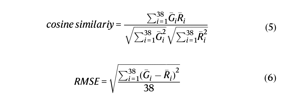
Filtering out impossible biology

• Not all generated data is valid, for example: white blood cell subtypes must sum to ~100% thus they included a filter that automatically removed any calculations that exceeded ~105%.
• They then measured accuracy using Cosine similarity → pattern similarity and RMSE → numerical error

Training and fine-tuning

• The dataset was split into 80% training data and 20% completely unseen compounds
• The model trained over thousands of iterations, stabilized around 1,000 epochs and ran until optimization around 6,000 epochs. This is when the model converged.

Stress-testing the model

• It was tested in different scenarios and it passed: It could assess compounds that were structurally different than what it was used to, it could predict effects for new drugs, and it could accurately predict the effects of the same drug across time. For example drugs tested before 1982 and the same studies conducted afterwards were used as the test data and the system was able to match accurately.

External validation: does it hold up?

The model was tested on a completely independent dataset: DrugMatrix, and the results were in ~83% agreement with real experimental outcomes. This is as consistent as different real datasets would be with each other.